Authored by Punit Arani

Supervised by Dr. Heni Ben Amor

Code: github.com/punitarani/cellular-sp500

This is not Financial Advice but rather a fun way to learn about the intersection of Cellular Automata and Neural Networks for Stock Market Simulation.

Abstract

Predicting stock market behavior is a complex task due to its non-linear and non-stationary dynamics. Traditional modeling methods often fall short in capturing these complexities. This paper proposes a novel approach to simulate the S&P 500 index by integrating Cellular Automata (CA) and Long Short-Term Memory (LSTM) neural networks. By representing stocks as cells on a grid and modeling their interactions with CA rules informed by LSTM predictions, we aim to capture both spatial and temporal dependencies in stock price movements. We utilize hierarchical clustering and market capitalization weighting for grid placement to reflect the inherent relationships and significance of stocks within the index. Our results demonstrate that this hybrid approach effectively groups stocks with similar behaviors and industries, providing a promising direction for simulating and understanding complex financial systems.

Introduction

The stock market is a highly complex system characterized by intricate interdependencies and dynamic behaviors. Traditional modeling techniques, such as stochastic processes and regression analyses, often struggle to encapsulate the non-linear and non-stationary nature of market dynamics. This limitation necessitates the exploration of alternative modeling approaches.

Cellular Automata (CA) offer a discrete computational model capable of simulating complex systems through simple, local interaction rules. When combined with the predictive power of Long Short-Term Memory (LSTM) neural networks—a type of Recurrent Neural Network (RNN) adept at modeling sequence data and learning long-term dependencies—there is potential to create a robust framework for simulating stock market behaviors.

In this paper, we propose a novel methodology that integrates CA and LSTM neural networks to simulate the S&P 500 index. Each stock is represented as a cell on a grid, with its state determined by intraday price changes. The CA rules governing state transitions are informed by LSTM models trained on historical stock data, enabling the simulation to capture both the temporal dependencies and the spatial relationships between stocks.

Background

Cellular Automata

Cellular Automata are computational models consisting of a grid of cells, each of which can be in a finite number of states. The state of each cell evolves over discrete time steps according to a set of rules that depend on the states of neighboring cells. CA have been successfully applied in various fields such as physics, biology, and social sciences to model complex phenomena.

Long Short-Term Memory Networks

LSTM networks are a type of RNN designed to overcome the limitations of traditional RNNs, particularly the vanishing gradient problem. They are capable of learning long-term dependencies in sequence data by maintaining a memory cell and employing gating mechanisms to control the flow of information. This makes LSTMs suitable for modeling time-series data with complex temporal dynamics, such as stock prices.

Methodology

Data Preparation

We utilized historical daily percentage change data for 500 stocks within the S&P 500 index. To create an evenly sized grid (20 rows × 25 columns), we excluded the three smallest-cap stocks, resulting in a total of 500 stocks for our simulation.

Correlation Matrix and Hierarchical Clustering

A correlation matrix was computed using the daily percentage changes, representing the pairwise correlations between stocks. Hierarchical clustering was then performed on this matrix using Ward's method, which minimizes the variance within clusters.

The clustering process involved the following steps:

1. Distance Matrix Calculation: We converted the correlation matrix into a distance matrix by subtracting the absolute correlation values from 1. This distance matrix was then transformed into a condensed format using scipy.spatial.distance.squareform, as required by the clustering algorithm.

2. Hierarchical Clustering: Using scipy.cluster.hierarchy.linkage, we performed hierarchical clustering on the distance matrix. We chose Ward's method for its variance-minimizing approach, which aims to create compact and homogeneous clusters. This method is similar to k-means in its objective but allows for a hierarchical structure.

3. Dendrogram Creation: The resulting linkage matrix was used to create a dendrogram, visualizing the hierarchical relationships between stocks. While the full dendrogram for 500 stocks is complex, it provides valuable insights into the clustering structure.

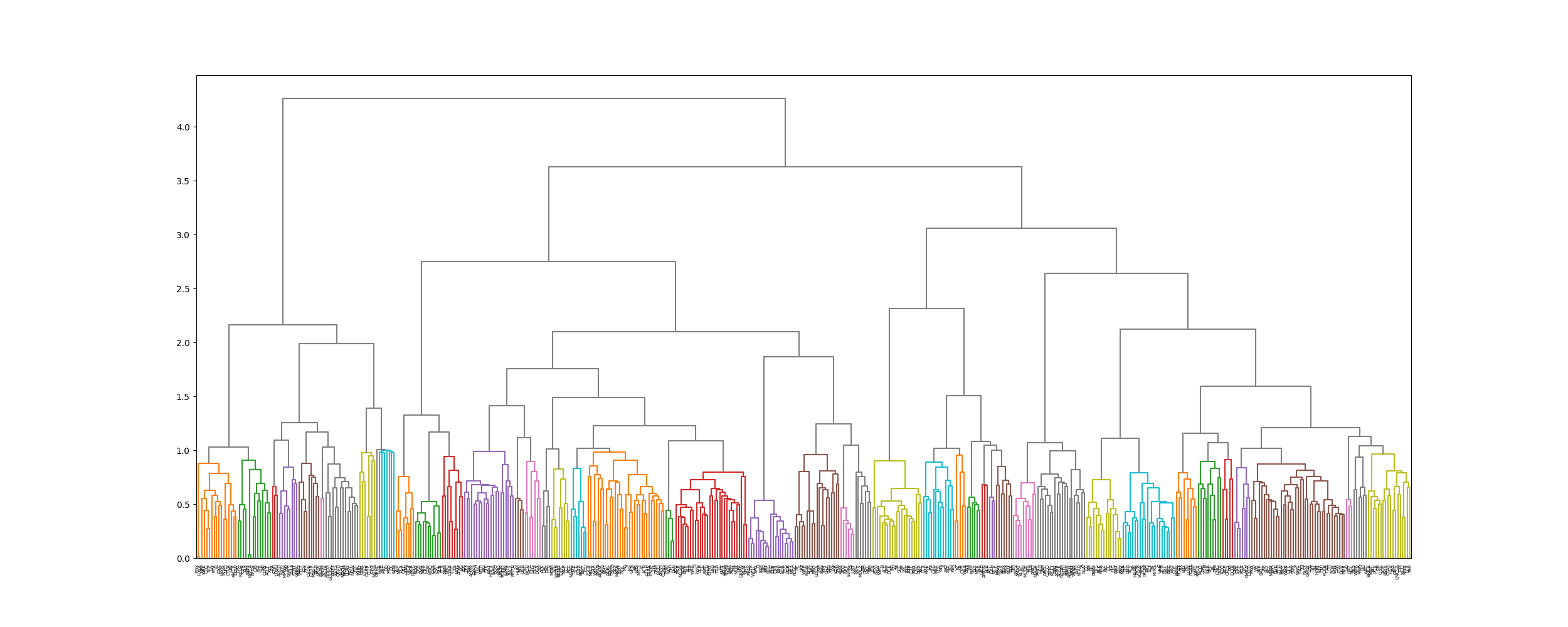
The optimal number of clusters was determined by maximizing a combined score of the silhouette coefficient and cluster size distribution, resulting in 16 clusters. This approach balanced cluster cohesion with a reasonable distribution of cluster sizes, providing an effective grouping for our stock market simulation.

Clustering Evaluation

To determine the optimal number of clusters, we employed a combination of the silhouette coefficient and cluster size distribution. The process involved cutting the dendrogram at various heights using scipy.cluster.hierarchy.fcluster, with the criterion parameter set to maxclust to specify the maximum number of clusters through the t parameter.

We tested different values of t between 5 and 20, calculating the silhouette score for each. The silhouette score measures how similar an object is to its own cluster compared to other clusters, ranging from -1 to 1, with higher scores indicating better clustering.

Additionally, we considered the distribution of cluster sizes to ensure a balanced grouping. A combined score was calculated, taking into account both the silhouette coefficient and the evenness of cluster size distribution.

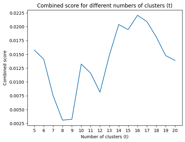
The evaluation resulted in an optimal t value of 16, yielding the highest combined score of 0.022. This balance between cluster cohesion and size distribution provided the most effective grouping for our stock market simulation.

Grid Placement Strategy

Stocks were placed on a 2D grid based on their cluster assignments and market capitalizations. The grid placement aimed to reflect the relationships between stocks, with more highly correlated stocks placed closer together. Market capitalization weighting ensured that larger-cap stocks, which have a greater influence on the S&P 500 index, were positioned centrally.

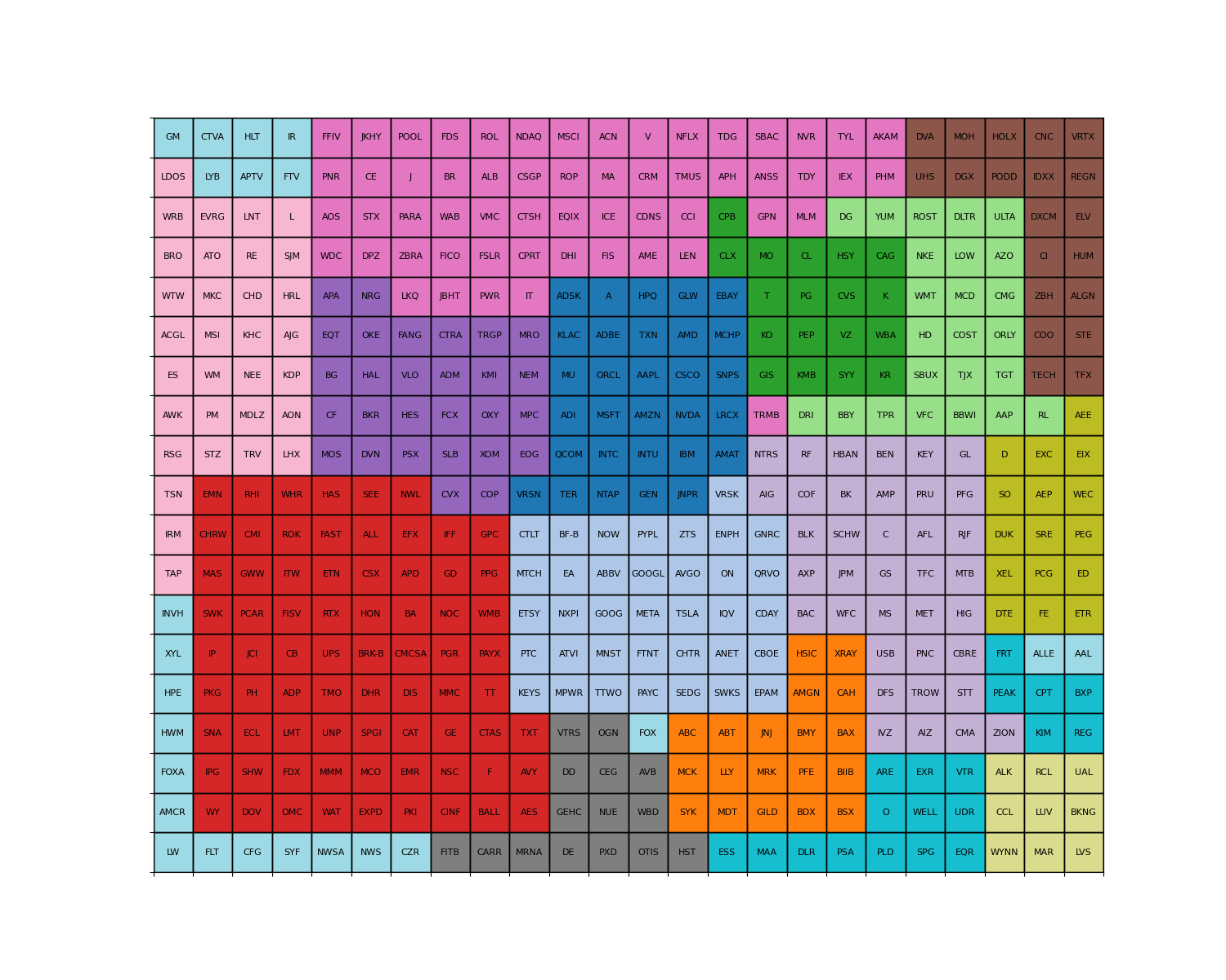
Placement Evaluation

An evaluation function was developed to assess the quality of the grid placement. The function penalized placements where stocks with larger market capitalizations were placed further from the grid center, promoting a configuration where influential stocks are centrally located.

The evaluation process involved:

1. Calculating the grid center and maximum market capitalization.
2. Iterating through each grid cell, computing a score based on the stock's market cap weight and distance from the center.
3. Summing these scores to produce a total placement score, with lower scores indicating better placements.

Force-Directed Graph Layout

A force-directed graph layout was employed to optimize the spatial positions of stocks on the grid. Stocks were modeled as nodes in a weighted graph, with edge weights representing the inverse of the absolute correlations. The spring layout algorithm from NetworkX was used to position the nodes, balancing attractive forces (correlations) and repulsive forces (node separation).

Placement Strategy

The optimal grid placement was determined through an iterative process:

1. Generate random placements for each cluster of stocks.
2. Evaluate each placement using the evaluation function.
3. Retain the placement with the lowest score.
4. Repeat for a specified number of iterations (10,000 in the full implementation).

This approach ensured a balance between cluster cohesion and the central positioning of high-impact stocks.

LSTM Model Training

Individual LSTM models were trained for each stock using sequences of 5-day historical percentage changes. The input to each model was a sequence of the previous 4 days, and the target was the percentage change on the 5th day. The models aimed to capture the temporal dependencies in stock price movements.

Model Architecture

The LSTM model was implemented using PyTorch, with the following key components:

1. Input layer: Accepts a single feature (daily percentage change)
2. LSTM layer: Processes the input sequence
3. Fully connected layer: Maps the LSTM output to the final prediction

The model's forward pass processes the input tensor of shape (batch_size, seq_len, input_size) through the LSTM and fully connected layers, outputting a tensor of shape (batch_size, output_size).

Training Process

The training process involved:

1. Dividing historical data into 5-day sequences
2. Using the first 4 days as input features and the 5th day as the target label
3. Training the LSTM model to learn the relationship between input sequences and target labels

This 5-day window was chosen to capture short-term dependencies and weekly patterns in stock price movements.

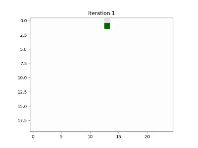
Simulation using Cellular Automata

The CA simulation was conducted by integrating the LSTM models into the state transition rules. For each stock (cell), the LSTM model predicted the next state based on its historical data and the states of its neighboring stocks. The simulation iteratively updated the grid, propagating the effects of individual stock movements throughout the network.

Prediction Algorithm

A breadth-first search (BFS) approach was used to simulate the spread of price changes across the grid. Starting from a chosen stock, the algorithm predicted the next state of its neighbors using the LSTM models, then proceeded to predict the neighbors of those neighbors, and so on, until the entire grid was updated.

The simulation process involved:

1. Initializing a queue with the starting stock and its input sequence
2. Dequeuing stocks, predicting their neighbors' states using LSTM models
3. Enqueueing unvisited neighbors with updated input sequences
4. Continuing until all stocks in the grid were visited

This approach effectively modeled the entire cellular automata, capturing complex interactions between stocks and leveraging both learned temporal dependencies and spatial relationships.

Results

Clustering Analysis

The hierarchical clustering algorithm effectively grouped stocks with similar behaviors and industries, as evidenced by the composition of the clusters. For example:

• Cluster 13 predominantly contained technology stocks like Apple (AAPL), Microsoft (MSFT), and NVIDIA (NVDA).
• Cluster 14 included major bank stocks such as JPMorgan Chase (JPM), Bank of America (BAC), and Citigroup (C).
• Cluster 7 comprised travel stocks, including airlines (AAL, DAL), cruise lines (CCL, RCL), and hotels (MAR, MGM).

Grid Placement Evaluation

The grid placement strategy successfully positioned larger-cap stocks near the center of the grid, reflecting their greater influence on the index. The evaluation function’s score indicated a well-optimized placement, balancing cluster cohesion and market capitalization weighting.

Simulation Outcomes

The CA simulation, incorporating the LSTM models, generated plausible stock price movements over the simulated period. The integration of temporal and spatial dependencies allowed the model to capture complex interactions between stocks, providing insights into the propagation of market dynamics.

Case Study: Apple Inc. (AAPL)

Simulating a 0.5% increase in Apple’s stock price, the model predicted subsequent changes in neighboring technology stocks due to their high correlation and proximity on the grid. This demonstrates the model’s ability to simulate the ripple effects of price changes across related stocks.

Discussion

The proposed methodology demonstrates the potential of combining cellular automata with LSTM neural networks for simulating stock market behaviors. By leveraging the strengths of both approaches—CA’s ability to model spatial interactions and LSTM’s capacity for capturing temporal dependencies—we can create a more comprehensive model of the stock market.

The clustering results validate the assumption that stocks within the same industry or sector exhibit similar behaviors. This clustering informed the grid placement, enhancing the realism of the simulation.

However, limitations exist. The model’s accuracy is contingent on the quality and quantity of historical data, and the assumption that past patterns will continue into the future may not always hold. Additionally, the computational complexity of training individual LSTM models for each stock may be substantial.

Conclusion

This paper presents a novel approach to simulating the S&P 500 index by integrating cellular automata and LSTM neural networks. The methodology effectively captures both the temporal dynamics of individual stocks and the spatial interactions between them. The results indicate that this hybrid model can provide valuable insights into stock market behaviors, with potential applications in financial analysis and decision-making processes.

Future Work

Future research could explore the incorporation of additional factors, such as macroeconomic indicators or news sentiment analysis, to enhance the model’s predictive capabilities. Additionally, optimizing the computational efficiency of the model and exploring alternative neural network architectures may further improve performance.

Appendix

Code: github.com/punitarani/cellular-sp500

Notebook: SP500-Cellular-Automata.ipynb

Demo

Usage

Requirements

• Python 3.10
• Poetry

Installation

poetry install

Running the Simulator

python simulator.py --ticker <STR> --change <FLOAT>

You can also simply pass the arguments without --ticker and --change as long as they are passed in order.

To run with default arguments (AAPL and 0.245)

python simulator.py

To run with custom arguments (MSFT and -0.147)

python simulator.py MSFT -0.147

This will run the simulator by using the previous 4 days of real data, and then setting the 5th day change for the provided stock ticker before simulating the performance of the other stocks.

NOTE: Running the simulator for the first time can take 10-30s to set up. Each simulation takes 5-15s.

Downloading Latest Data

Update the start_date and end_date in data.py to the desired date range. The default is 1st Jan 1990 to 31st Dec 2022.

4 Million Data Points over 33 years for 503 stocks in the S&P 500.

Then run the following command:

python data.py

This will perform the following steps:

1. Get the latest list of stocks in the S&P 500 from Wikipedia
2. Downloads the historical data for each stock from Stooq using pandas-datareader

• Uses multiprocessing to speed up the download but can take ~2-5 minutes
• Use any applicable data source for pandas-datareader by updating data = web.DataReader(ticker, 'stooq', start_date, end_date) in get_stock_data()
• Saves the data to data/<TICKER>.parquet. Uses parquet format for faster read/write times.

3. Downloads the latest market capitalization data from Yahoo Finance and saves it to sp500_market_caps.json

Generating the grid

To find the optimal grid positions for each stock, run the following command:

python grid.py

This saves the grid positions to sp500_grid.csv.

The script performs the following:

1. Load the historical data for all stocks
2. Performs hierarchical clustering on the stocks based on their correlation
3. Creates a force-directed graph to find the optimal grid positions for each stock
4. Performs an evaluation of the grid positions by checking cluster tightness and concentrating larger market cap stocks in the center of the grid
5. Repeat steps 3 and 4 for 10000 iterations while evaluating the positions to find the best grid placement

Training the Neural Network

To train the LSTM models for grid weights, run the following command:

python train.py

This will train the LSTM models for each neighboring stock pair and save the weights to weights/<TICKER>.pth, the model to models/<TICKER>.pt and scalers to scalers/<TICKER>/.pkl

The models are trained on sequences of 5 consecutive days. This was chosen because it is inefficient and impractical to train on shorter sequences because it is hard to make predictions on a single day's data. Similarly, it is inefficient to train on longer sequences because the number of possible sequences increases exponentially and the prediction complexity increases with the sequence length.

This is a very computationally expensive process. It took over 7 hours on a 4 core machine with 16 GB RAM laptop and over 3 hours on a 16 core server instance. Currently, the models are trained on CPU only as there are issues training PyTorch LSTM models on GPU.

Notes

Using the LSTM Models without the Simulator

The LSTM models can be used without the simulator by using calling the LSTMModel class directly.

Using the provided load_model_and_scaler, the models and scalers can be loaded from the saved files.

from train import load_model_and_scaler
 
# Load the trained models and scalers for AAPL and ORCL
model_AAPL, scaler_AAPL = load_model_and_scaler("model_A_AAPL-ORCL")
model_ORCL, scaler_ORCL = load_model_and_scaler("model_B_AAPL-ORCL")

Then, we can use the predict method to make predictions for a given input sequence. The input sequence should be a numpy array of shape (5, 1) because the models were trained on 5 day sequences.

The inputs must be a percentage change from the previous day's closing price. The percentage must be represented as a decimal and not a percentage. Example: 1.23% as 1.23 not 0.0123.

import numpy as np
 
# Example input sequences for AAPL and ORCL
input_seq_AAPL = np.array([[2.1234], [-1.4567], [3.2456], [1.2345], [-2.0987]])
input_seq_ORCL = np.array([[1.3456], [-2.3456], [3.1234], [2.4567], [-1.2345]])
 
prediction_AAPL = model_AAPL.predict(scaler_AAPL, input_seq_AAPL)
prediction_ORCL = model_ORCL.predict(scaler_ORCL, input_seq_ORCL)
 
print(f"AAPL Prediction: {prediction_AAPL:.4f}")
print(f"ORCL Prediction: {prediction_ORCL:.4f}")

AAPL Prediction: 0.2831
ORCL Prediction: 0.0279

Using real data

Assuming the latest data has been downloaded, we can use the get_trailing_stock_data from simulator.py to get the previous days' data.

from simulator import get_trailing_stock_data
 
# Get the previous day's data for AAPL and ORCL
input_seq_AAPL = get_trailing_stock_data("AAPL", -3.5625)
input_seq_ORCL = get_trailing_stock_data("ORCL", -2.7492)
# This will use the previous 4 days' data followed by the input value (second argument)